The One-Transition and Two-Transition Approximations

The most complicated part of the conditional aggregate mean transform $\hat{M}(s\vert {\bf j}, {\bf x})$ in (24) is the matrix inverse $(I-\hat{q}(s))^{-1}$ in the transform of the single-source transition probability in (14). Since the matrix inverse calculation can be a computational burden when the number of levels is large, it is natural to seek approximations which avoid this matrix inverse. We describe such approximations in this section.

The matrix inverse (I-q(s))^-1 is a compact representation for the series $\sum_{n=0}^\infty q(s)^n$.For P(t|x), it captures the possibility of any number of transitions up to time t. However, if the levels are relatively long in the time scale relevant for control, then the mean for times t of interest will only be significantly affected by a very few transitions. Indeed, often only a single transition need be considered.

The single-transition approximation is obtained by making the Markov chain absorbing after one transition. Hence, the single-transition approximation is simply  

$$P_{jk} (t\vert x) \approx H_{jk} (t\vert x) ~, \quad j \ne k... ... P_{jj} (t\vert x) \approx G_j^c (t\vert x) + H_{jj} (t\vert x)$$ (22)

for H_jk (t|x) in (9) and G_j (t|x) in (9). From (25) we see that no inversion is needed.

Alternatively, we can develop a two-transition approximation. (Extensions to higher numbers are straightforward.) Modifying the proof of Theorem 2.1 in a straightforward manner, we obtain  

$$P_{jk} (t\vert x) = \int_0^t G_k^c (t-u) dH_{jk} (u\vert x) + \sum_\ell \int_0^t P_{\ell k} F_{lk} (t-u) dH_{j\ell} (u\vert x)$$ (23)

for $j \ne k$ and  

$$P_{jj} (t\vert x) = G_j^c (t\vert x) + \sum_\ell \int_0^t P_{\ell j} F_{lj} (t-u) dH_{j\ell} (u\vert x) ~.$$ (24)

Expressed in the form of transforms, (26) and (27) become  

$$\hat{P}_{jk} (s\vert x) = \hat{h}_{jk} (s\vert x) \displayst... ...l} (s\vert x) P_{\ell k} \displaystyle\frac{\hat{f}_{lk}(s)}{s}$$ (25)

for $j \ne k$ and  

$$\hat{P}_{jj} (s\vert x) = \displaystyle\frac{1- \hat{g}_j (s... ...l} (s\vert x) P_{lj} \displaystyle\frac{\hat{f}_{lj} (s)}{s} ~.$$ (26)

Numerical inversion can easily be applied with (28) and (29). However, since the time-domain formulas (26) and (27) involve single convolution integrals, numerical computation of (26) and (27) in the time domain is also a feasible alternative. Moreover, if the underlying distributions have special structure, then the integrals in (26) and (27) can be calculated analytically. For example, analytical integration can easily be done when all holding-time distributions are hyperexponential.

Example 3.1. To illustrate how the two approximations compare to the exact conditional mean, we give a numerical example. We consider a single source with four levels. The transitions move cyclically through the levels: P₁₂ = P₂₃ = P₃₄ = P₄₁ = 1. The level holding-time ccdf's are:

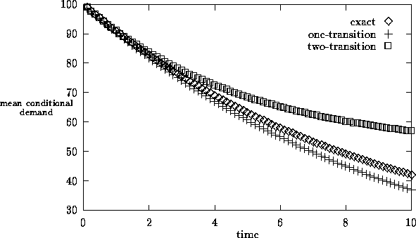
The level bandwidths are b₁ = b₃ = 100 and b₂ = b₄ = 0. Suppose that we start in level 1 with an age of 8. From the form of G₁^c (t), we see that the conditional level-1 holding-time ccdf G₁^c (t|x) is then approximately e^-0.1t. Hence the first two mean level holding times are approximately 10. Hence we might consider the one-transition and two-transition approximations in the interval [0,10]. The two approximations are compared to the exact value of the conditional mean in Figure 1. (All are computed by numerical transform inversion.) The approximations are very good up to t = 1 or 2, but they start to degrade by t = 10. The two-transition approximation performs not so well for larger t because the actual holding time in level 3 is likely to be quite short. More generally, our experience is that the one-transition and two-transition approximations tend to perform quite satisfactorily if the mean level holding times in the first few levels are substantially larger than the times t of interest. In this example the approximations are quite good in the interval [0,1].

  

Figure 1: A comparison of the one-transition and two-transition approximations with the exact conditional mean aggregate demand in Example 3.1.