The Value of Information

We can use the source model to investigate the value of information. We can consider how prediction is improved when we condition on, first, only the level and, second, on both level and age. The reference case is the steady-state mean  

$$M = \sum_{i=1}^n m^i \quad \mbox{and $m^i = \sum b_j^i p_j^i $}~,$$ (27)

where p_jⁱ is the steady-state probability, i.e.,  

$$p_j^i = \displaystyle\frac{\pi^i_j m(G^i_j )}{\sum_k \pi^i_k m(G^i_k )} ~,$$ (28)

with $\pi^i$ the steady-state vector of the Markov chain Pⁱ $(\pi^i = \pi^i P^i)$ and m(Gⁱ_j ) the mean of Gⁱ_j for G_j in (8), for all sources i. With the steady-state mean, there is no conditioning. Section 2 gives the formula for conditioning on both level and age. Now we give the formulas conditioning only on the level; i.e., we condition on the level, assuming that we are in steady-state. We omit the i superscript. Then the age in level j has the stationary-excess cdf  

$$G_{je} (t) = \displaystyle\frac{1}{m(G_j )} \int_0^t G_j^c (u) du ~, \quad t \geq 0 ~.$$ (29)

Let P_jk (t) be the probability of being in level k at time t conditional on being in level j in steady state at time 0. Let $\hat{P}_{jk} (s)$ be its Laplace transform. Let m_j (t) be the conditional steady-state mean given level j at time 0 and let $\hat{m}_j (s)$ be its Laplace transform: Clearly  

$$m_j (t) = \sum_{k=1}^J P_{jk} (t) b_k \quad \mbox{ and~~~ $\hat{m}_j (s) = \sum_{k=1}^J \hat{P}_{jk}(s) b_k$} ~.$$ (30)

Hence, it suffices to calculate $\hat{P}_{jk} (s)$.

Theorem 6936

 Assume that the level-holding-time cdf depends only on the originating level, i.e., F_jk (t) = G_j (t). The steady-state transition probabilities conditional on the level for a single SMP source have the matrix of Laplace transforms  

$$\hat{P}(s) = \hat{D}_e(s) + \hat{g}_e (s) \hat{P}(s\vert)~,$$ (31)

where $\hat{P}(s\vert)$ is the matrix in (14), $\hat{g}_e (s)$ is the matrix with elements  

$$\hat{g}_{ejk} (s) = P_{jk} \hat{g}_{je} (s) = P_{jk} \displaystyle\frac{(1- \hat{g}_j (s))}{sm(G_j )} ~,$$ (32)

$\hat{D}_e(s)$ is the diagonal matrix with diagonal elements  

$$\hat{D}_{ejj} (s) \equiv \displaystyle\frac{1-\hat{g}_{je}(s... ... = \displaystyle\frac{sm(G_j) -1+ \hat{g}_j (s)}{s^2 m(G_j )}~,$$ (33)

$\hat{g}_j (s)$ is the level-j holding-time LST and $\hat{g}_{je}(s)$ is the LST of its stationary-excess cdf in (32).

Proof. Modify the proof of Theorem 2.1, inserting P_jl G_je(t) for H_jl (t|x) and G_je^c (t) for G_j^c (t|x). Example 4.1. Consider the on-off source in Example 2.1. Paralleling (17), it suffices to calculate only P₁₂(t). Its Laplace transform is  

$$\hat{P}_{12} (s) = \displaystyle\frac{\hat{g}_{1e} (s) (1- \hat g_2 (s))}{s(1- \hat{g}_1 (s) \hat{g}_2 (s))} ~.$$ (34)

Example 4.2. To show the value of knowing the age, consider an on-off source with holding-time ccdf's  

$$G_1^c (t) = 0.01e^{-0.01t} + 0.1e^{-0.1t} + .89e^{-t},\qquad G_2^c (t) = e^{-t} ~,~~~ t \ge 0 ~.$$ (35)

Let the bandwidths be b₁ = 100 and b₂ = 0. Since m(G₁ ) = 2.89 and m(G₂ ) = 1.00, the steady-state mean is

$$EB( \infty) = \displaystyle\frac{100m(G_1 )}{m(G_1 ) + m(G_2 )} = 74.29 ~.$$

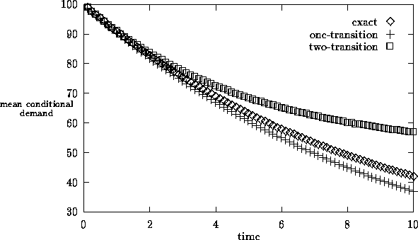
Let the initial level be 1. Since G₁ has an exponential component with mean 100, we anticipate the time to reach steady state to be between 100 and 1000. In Figure 2 we plot the conditional mean m₁ (t|x) for x = 0.5, 5.0 and 50.0, computed by numerical transform inversion. Figure 2 shows that the age plays a very important role.

  

Figure 2: The conditional mean aggregate demand as a function of the age of the holding time in level 1 for Example 4.2.