A Linear Approximation

Assuming that the relevant time is not too large, we might approximate the conditional mean bandwidth using a Taylor-series approximation

 

E(B(t)|B(0) = x) = x + tr (x) ,

where

$$r(x) := E(B'(0) \vert B (0) = x) = \sum_{i=1}^n \sum_{j=1}^... ...{p}_j^i \sum_{k=1}^{J_i} P_{jk} (b_k^i - b_j^i ) / m(G_{j} ) ~,$$

which has the advantage that no numerical inversion is required.

Suppose the service capacity is c>E(B(0)) and we condition on B(0)>c. If r(B(0))<0, we can use (50) to approximate the first time to return to c, the recovery time, by  

$$\tau = (x-c)/r(x) ~.$$ (45)

Suppose in addition that B is reversible; this will happen if the matrix P is reversible. Then since both the residual lifetime and the current age have distribution F_jke, $E(B(-t)\mid B(0))=E(B(t)\mid B(0))$.Consequently B(0)=x is a local maximum, at t=0, of $E(B(t)\mid B(0))$.

Now suppose that there are n independent sources. Then as in [10], it follows by use of an appropriate functional law of large numbers that, as $n \rightarrow \infty$ under regularity conditions, the stochastic paths of the B process converge to this mean path. Thus we can identify, asymptotically as $n\to\infty$, t=0 as a hitting time for the level x. Thus, we can use (43) to approximate the probability of this hitting time and $\tau$ in (51) to approximate the associated recovery time.
Example 7.1. Consider homogeneous two-level sources, i.e., $j\in\{1,2\}$, $0\le b_1 < b_2$, p₁+p₂=1 with mean lifetimes m₁,m₂, and P₁₁=P₂₂=1-P₁₂=1-P₂₁=0. With n sources and B(0)=x we can calculate the $\bar p_j$ in (47) directly from the relation $x=n (\bar p_1 b_1 + \bar p_2 b_2)$for $x\in \{nb_1,(n-1)b_1+b_2,\ldots,b_1+(n-1)b_2,nb_2\}$. Then

As a concrete example, we let b₁=1, b₂=5, m₁=3, m₂=1, giving a mean bandwidth per source of (m₁b₁+m₂b₂)/(m₁+m₂)=2. We also let n = 50 and c = 150. The parameters of the example were chosen as a caricature of video traffic on an OC3 link: take b_i , x, c in Mb/sec, m_i in seconds.

 

$$\tau$$ 2|c| # sources initial steady-state

2|c|initially in total probability 2c|inversion

2|c|each level demand of x linear exponential Pareto

n₁ n₂ x e^-I(x) approx. duration duration

$$7.5\times 10^{-4}$$ 25 25 150

$$1.9\times 10^{-5}$$ 22 28 162 0.15 0.16 0.19

$$2.4\times 10^{-7}$$ 19 31 174 0.24 0.29 0.41

$$1.4\times 10^{-9}$$ 16 34 186 0.31 0.41 0.64

$$3.5\times 10^{-12}$$ 13 37 198 0.37 0.50 0.91

We present in Table 1 some values of n₁ , n₂, the number of sources in each level for a given x, the approximate probability e^-I(x) of demand exceeding x (using I from (45)), and $\tau$. For comparison we give also the exact recovery time for the mean, calculated by using numerical transform inversion methods [1], for particular models of level durations with the same means: (i) both level durations exponentially distributed; (ii) lower level exponential, upper level duration Pareto with exponent 1.5, and hence ccdf G^c(x)=(1+2x)^-3/2 in order to give mean m₂=1. The Pareto density g(x) = a(1+x)^-(1+a) has Laplace transform $ae^s s^a \Gamma (-a, s)$, where $\Gamma (a,z)$is the incomplete gamma function  

$$\Gamma (a,z) = \int_z^\infty t^{a-1} e^{-t} dt ~.$$ (46)

Hence, the required transform values for the Pareto distribution are readily computable.

  

Figure 3: Recovery curves for two-level sources: linear approximation and numerical transform inversion with exponential and Pareto durations in the higher level; see Example 7.1.

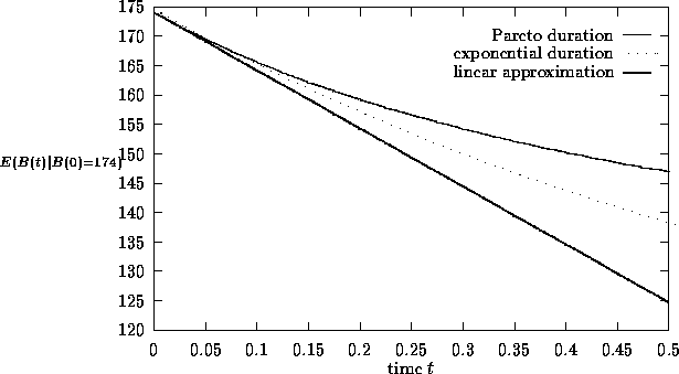In Figure 3 we display the evolution of the conditioned mean in the linear approximation, and for the two distributions above with the same mean. As should be expected, the linear approximation is more accurate when the initial level x is closer to the capacity c. The linear approximation also behaves worse for the Pareto high-level durations than for the exponential high-level durations. The linear approximation tends to consistently provide a lower bound on the true recovery time for the mean. Even though the linear-approximation estimate of the recovery time diverges from the true mean computed by numerical inversion as the hitting level x increases, the probability of such high x can be very small. Even the largest errors in predicted recovery times in Table 1 are within one order of magnitude, and so might be regarded as suitable approximations. >From our experiments, we conclude that the linear approximation is a convenient rough approximation, but that the numerical inversion yields greater accuracy.

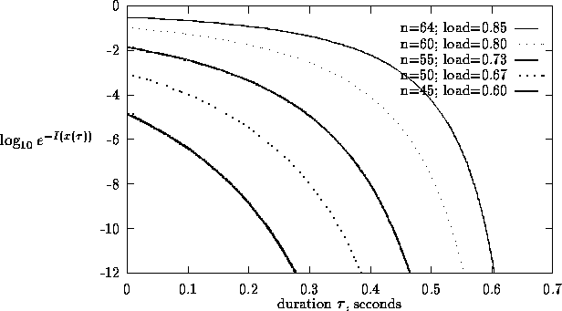
Simple criteria for link dimensioning. A key point is the two-dimensional characterization of rare congestion events in terms of likelihood and recovery time. To further show how this perspective can be exploited, we plot in Figure 4, for various offered loads, the approximate probability $e^{-I(x(\tau))}$ of a demand at least $x(\tau)$ as a function of $\tau$, where $\tau=(c-x(\tau))/r(x(\tau))$; i.e., $x(\tau)$ is the demand from which the recovery time to the level c is $\tau$, using the linear approximation. Figure 4 shows that the two criteria together impose more constraints on what sets of sources are acceptable. Expressed differently, for the same probability of occurrence, rare congestion events can have very different recovery times.

  

Figure 4: Design criteria: estimated probability of overdemand of at least duration $\tau$, for various offered loads; see Section 7.